Download the notebook here!
Interactive online version: ![]()
Optimal Replacement of GMC Bus Engines: An empirical model of Harold Zurcher
This notebook replicates the descriptives in Tabla IIa and IIb from > Rust, J. (1987). Optimal Replacement of GMC Bus Engines: An empirical model of Harold Zurcher. Econometrica, Vol. 55, No.5, 999-1033.
The data is taken from the NFXP software provided by Rust which is available to download here.
Preparations
Before executing this file the raw data needs to be processed.
[7]:
import os
import sys
import numpy as np
import pandas as pd
import matplotlib.pyplot as plt
from scipy.signal import savgol_filter

sys.path.insert(0, "../data/")
from data_processing import data_reading  # noqa: E402
from data_processing import get_data_storage  # noqa: E402
[4]:
data_reading()
Odometer at Engine Replacement
Table IIa in Rust’s paper describes the milage on which a engine replacement occured. As there are buses, which had a second replacement during the time of the observation, the record of the second replacement will be reduced by the milage of the first, to get the real life time milage of an engine.
[5]:
data_path = get_data_storage()
dict_df = dict()
for filename in os.listdir(data_path + "/pkl/group_data/"):
    if filename.endswith(".pkl"):
        dict_df[filename[0:7]] = pd.read_pickle(
            data_path + "/pkl/group_data/" + filename
        )
[6]:
df = pd.DataFrame()
for j, i in enumerate(sorted(dict_df.keys())):
    df2 = dict_df[i][["Odo_1"]][dict_df[i]["Odo_1"] > 0]
    df2 = df2.rename(columns={"Odo_1": i})
    df3 = dict_df[i][["Odo_2"]].sub(dict_df[i]["Odo_1"], axis=0)[
        dict_df[i]["Odo_2"] > 0
    ]
    df3 = df3.rename(columns={"Odo_2": i})
    df3 = df3.set_index(df3.index.astype(str) + "_2")
    df4 = pd.concat([df2, df3])
    if j == 0:
        df = df4.describe()
    else:
        df = pd.concat([df, df4.describe()], axis=1)
df = df.transpose()
df.fillna(0).astype(int)
[6]:
| count | mean | std | min | 25% | 50% | 75% | max | |
|---|---|---|---|---|---|---|---|---|
| group_1 | 0 | 0 | 0 | 0 | 0 | 0 | 0 | 0 |
| group_2 | 0 | 0 | 0 | 0 | 0 | 0 | 0 | 0 |
| group_3 | 27 | 199733 | 37459 | 124800 | 174550 | 204800 | 230650 | 273400 |
| group_4 | 33 | 257336 | 65477 | 121300 | 215000 | 264100 | 292400 | 387300 |
| group_5 | 11 | 245290 | 60257 | 118000 | 229600 | 250600 | 282250 | 322500 |
| group_6 | 7 | 150785 | 61006 | 82400 | 107450 | 125500 | 197750 | 237200 |
| group_7 | 27 | 208962 | 48980 | 121000 | 178650 | 207700 | 237200 | 331800 |
| group_8 | 19 | 186700 | 43956 | 132000 | 162900 | 182100 | 188400 | 297500 |
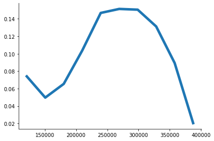
[7]:
i = "group_4"
df_group_4_rep_1 = dict_df[i][["Odo_1"]][dict_df[i]["Odo_1"] > 0]
df_group_4_rep_1 = df_group_4_rep_1.rename(columns={"Odo_1": i})
df_group_4_rep_2 = dict_df[i][["Odo_2"]].sub(dict_df[i]["Odo_1"], axis=0)[
    dict_df[i]["Odo_2"] > 0
]
df_group_4_rep_2 = df_group_4_rep_2.rename(columns={"Odo_2": i})
df_group_4_rep_2 = df_group_4_rep_2.set_index(df3.index.astype(str) + "_2")
df_group_4 = pd.concat([df_group_4_rep_1, df_group_4_rep_2])
[8]:
bins = 10
hist_data = np.histogram(df_group_4["group_4"].to_numpy(), bins=bins)
hist_data
[8]:
(array([2, 3, 1, 4, 3, 8, 6, 3, 1, 2]),
 array([121300., 147900., 174500., 201100., 227700., 254300., 280900.,
        307500., 334100., 360700., 387300.]))
[9]:
hist_normed = hist_data[0] / sum(hist_data[0])
x = np.linspace(np.min(hist_data[1]), np.max(hist_data[1]), bins)
hist_filter = savgol_filter(hist_normed, 9, 3)

fig, ax = plt.subplots(1, 1)
ax.plot(x, hist_filter)
[9]:
[<matplotlib.lines.Line2D at 0x7f28ad2eb310>]
Never failing buses
Table IIb explores buses, which never had an engine replacement. Therefore this data is left-censored, as the econometrican never observes the time of replacement. The table shows the variation in the odometer record at the end of the observation period.
[10]:
df = pd.DataFrame()
for i in sorted(dict_df.keys()):
    df2 = dict_df[i][[dict_df[i].columns.values[-1]]][dict_df[i]["Odo_1"] == 0]
    df2 = df2.rename(columns={df2.columns.values[0]: i})
    if j == 0:
        df = df2.describe()
    else:
        df = pd.concat([df, df2.describe()], axis=1)
df = df.transpose()
df = df.drop(df.columns[[4, 5, 6]], axis=1)
df[["max", "min", "mean", "std", "count"]].fillna(0).astype(int)
[10]:
| max | min | mean | std | count | |
|---|---|---|---|---|---|
| group_1 | 120151 | 65643 | 100116 | 12929 | 15 |
| group_2 | 161748 | 142009 | 151182 | 8529 | 4 |
| group_3 | 280802 | 199626 | 250766 | 21324 | 21 |
| group_4 | 352450 | 310910 | 337221 | 17802 | 5 |
| group_5 | 326843 | 326843 | 326843 | 0 | 1 |
| group_6 | 299040 | 232395 | 265263 | 33331 | 3 |
| group_7 | 0 | 0 | 0 | 0 | 0 |
| group_8 | 0 | 0 | 0 | 0 | 0 |